Linear Regression Model and Gradient Descent Algorithm

Blog

January 17, 2026

Univariate Linear Regression and Gradient Descent Method

Suppose we have a sample dataset \((x^{(i)},y^{(i)}),i=1,2,...,m\) as shown in the figure below:

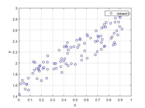
Univariate Linear Regression Dataset

It is obvious that \(y\) is linearly correlated with \(x\) . We establish a linear regression model between \(y\) and \(x\) , where \(x\) is the feature variable, and the hypothesis function is defined as:

\[h_\theta(x)=\theta_0+\theta_1x\]

The cost function is given by:

\[J(\theta_0,\theta_1)=\frac{1}{2m}\sum_{i=1}^{m}(h_\theta(x^{(i)})-y^{(i)})^2\]

To determine the model parameters that minimize the cost function, a commonly used method is the gradient descent method.

The steps of the gradient descent algorithm are as follows:

Make an initial guess for the model parameters \(\theta_0\) and \(\theta_1\) , regardless of their initial appropriateness.
Calculate the partial derivatives of \(J\) with respect to the two parameters \(\theta_0\) and \(\theta_1\) , multiply them by a suitable learning rate \(\alpha\) , and use these values as the driving force for parameter updates:

\[\theta_0:=\theta_0-\alpha\frac{\partial}{\partial \theta_0}J(\theta_0,\theta_1)=\theta_0-\alpha\frac{1}{m}\sum_{i=1}^{m}(\theta_0+\theta_1x^{(i)}-y^{(i)})\]\[\theta_1:=\theta_1-\alpha\frac{\partial}{\partial \theta_1}J(\theta_0,\theta_1)=\theta_1-\alpha\frac{1}{m}\sum_{i=1}^{m}(\theta_0+\theta_1x^{(i)}-y^{(i)})x^{(i)}\]

Compute the value of the cost function \(J\) after updating the parameters:

\[J(\theta_0,\theta_1)=\frac{1}{2m}\sum_{i=1}^{m}(\theta_0+\theta_1x^{(i)}-y^{(i)})^2\]

Check whether the change in \(J\) before and after parameter update is sufficiently small. If the magnitude of the change exceeds the convergence threshold, repeat steps 2 to 4 for iteration until the change in \(J\) is less than the convergence threshold. At this point, \(\theta_0\) and \(\theta_1\) are the optimal model parameters.

Organize the dataset into the following matrix form:

\[X=\begin{bmatrix} x^{(1)} \\ \vdots \\ x^{(m)} \end{bmatrix}\in\mathbb{R}^{m\times1}\]

\[Y=\begin{bmatrix} y^{(1)} \\ \vdots \\ y^{(m)} \end{bmatrix}\in\mathbb{R}^{m\times1}\]

The code implementation of the above iterative convergence process is as follows:

theta_0 = 0;
theta_1 = 0;
J = 1/(2*m)*sum((theta_0+theta_1.*X-Y).^2);
alpha = 1e-6;
while 1
    theta_0_tmp = theta_0-alpha/m*sum(theta_0+theta_1.*X-Y);
    theta_1_tmp = theta_1-alpha/m*sum((theta_0+theta_1.*X-Y).*X);
    J_tmp = 1/(2*m)*sum((theta_0_tmp+theta_1_tmp.*X-Y).^2);
    delta_J = J_tmp-J;
    theta_0 = theta_0_tmp;
    theta_1 = theta_1_tmp;
    J = J_tmp;
    if abs(delta_J)<=1e-12
        break
    end
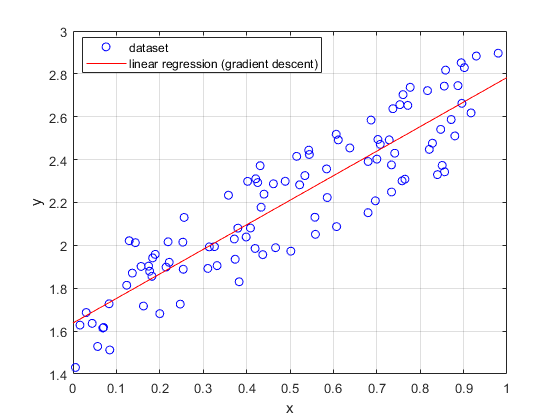
end

After convergence, we obtain the final model parameters \(\theta_0\) and \(\theta_1\) . The result of the univariate linear regression is shown in the figure below:

Univariate Linear Regression

Bivariate Linear Regression

Consider a more complex dataset \((x_1^{(i)},x_2^{(i)},y^{(i)}),i=1,2,...,m\) as shown in the figure below:

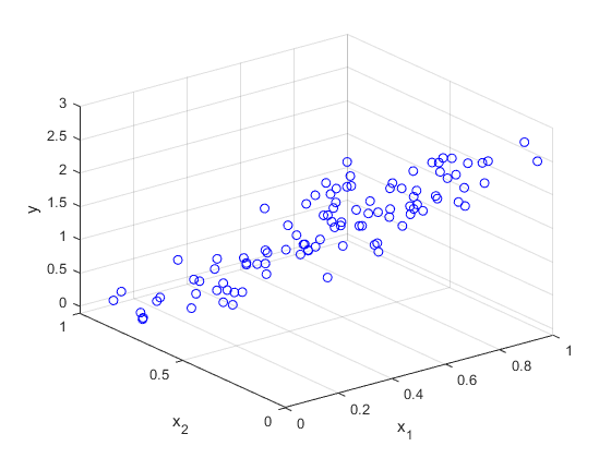
Bivariate Linear Regression Dataset

In this dataset, \(y\) is linearly correlated with both \(x_1\) and \(x_2\) . We establish a linear regression model between \(y\) and the two features, where \(x_1\) and \(x_2\) are the feature variables, and the hypothesis function is:

\[h_\theta(x)=\theta_0+\theta_1x_1+\theta_2x_2\]

The cost function is:

\[J(\theta_0,\theta_1,\theta_2)=\frac{1}{2m}\sum_{i=1}^{m}(h_\theta(x^{(i)})-y^{(i)})^2=\frac{1}{2m}\sum_{i=1}^{m}(\theta_0+\theta_1x_1^{(i)}+\theta_2x_2^{(i)}-y^{(i)})^2\]

Similar to univariate linear regression, we use the gradient descent algorithm to converge to the minimum value of \(J(\theta_0,\theta_1,\theta_2)\) .

During the gradient descent iteration, the parameter update rules are similar to those of univariate linear regression:

\[\theta_0:=\theta_0-\alpha\frac{\partial}{\partial \theta_0}J(\theta_0,\theta_1,\theta_2)=\theta_0-\alpha\frac{1}{m}\sum_{i=1}^{m}(\theta_0+\theta_1x_1^{(i)}+\theta_2x_2^{(i)}-y^{(i)})\]

\[\theta_1:=\theta_1-\alpha\frac{\partial}{\partial \theta_1}J(\theta_0,\theta_1,\theta_2)=\theta_1-\alpha\frac{1}{m}\sum_{i=1}^{m}(\theta_0+\theta_1x_1^{(i)}+\theta_2x_2^{(i)}-y^{(i)})x_1^{(i)}\]

\[\theta_2:=\theta_2-\alpha\frac{\partial}{\partial \theta_2}J(\theta_0,\theta_1,\theta_2)=\theta_2-\alpha\frac{1}{m}\sum_{i=1}^{m}(\theta_0+\theta_1x_1^{(i)}+\theta_2x_2^{(i)}-y^{(i)})x_2^{(i)}\]

Organize the dataset into the following matrix form:

\[X=\begin{bmatrix} x_1^{(1)}&x_2^{(1)}\\ \vdots&\vdots\\ x_1^{(m)}&x_2^{(m)} \end{bmatrix}\in\mathbb{R}^{m\times2}\]

\[Y=\begin{bmatrix} y^{(1)} \\ \vdots \\ y^{(m)} \end{bmatrix}\in\mathbb{R}^{m\times1}\]

The code implementation of the gradient descent iteration process is as follows:

theta_0 = 0;
theta_1 = 0;
theta_2 = 0;
J = 1/(2*m)*sum((theta_0+theta_1.*X(:,1)+theta_2.*X(:,2)-Y).^2);
alpha = 1e-6;
while 1
    theta_0_tmp = theta_0-alpha/m*sum(theta_0+theta_1.*X(:,1)+theta_2.*X(:,2)-Y);
    theta_1_tmp = theta_1-alpha/m*sum((theta_0+theta_1.*X(:,1)+theta_2.*X(:,2)-Y).*X(:,1));
    theta_2_tmp = theta_2-alpha/m*sum((theta_0+theta_1.*X(:,1)+theta_2.*X(:,2)-Y).*X(:,2));
    J_tmp = 1/(2*m)*sum((theta_0_tmp+theta_1_tmp.*X(:,1)+theta_2_tmp.*X(:,2)-Y).^2);
    delta_J = J_tmp-J;
    theta_0 = theta_0_tmp;
    theta_1 = theta_1_tmp;
    theta_2 = theta_2_tmp;
    J = J_tmp;
    if abs(delta_J)<=1e-12
        break
    end
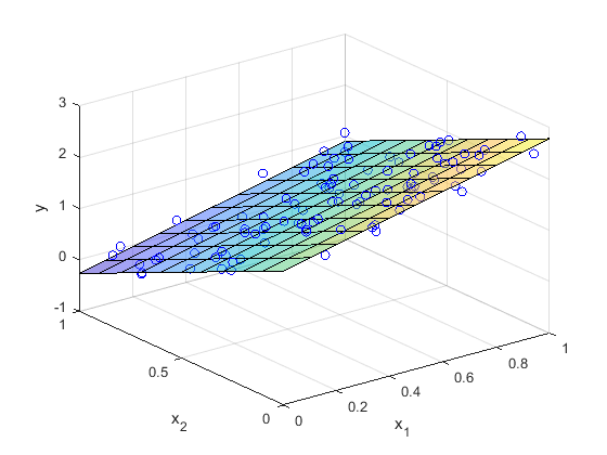
end

After convergence, we obtain the final model parameters \(\theta_0\), \(\theta_1\) and \(\theta_2\) . The result of the bivariate linear regression is shown in the figure below:

Bivariate Linear Regression

Multiple Linear Regression

We generalize the above concepts to a general multiple linear regression model. For a dataset \((x_1^{(i)},x_2^{(i)},\cdots,x_n^{(i)},y^{(i)}),i=1,2,...,m\) , we establish a multiple linear regression model with feature variables \(x_1,x_2,\cdots,x_n\) . The hypothesis function is:

\[h_\theta(x)=\theta_0+\theta_1x_1+\theta_2x_2+\cdots+\theta_nx_n\]

The cost function is:

\[J(\theta_0,\theta_1,\cdots,\theta_n)=\frac{1}{2m}\sum_{i=1}^{m}(h_\theta(x^{(i)})-y^{(i)})^2=\frac{1}{2m}\sum_{i=1}^{m}(\theta_0+\theta_1x_1^{(i)}+\cdots+\theta_nx_n^{(i)}-y^{(i)})^2\]

The parameter update rules during the gradient descent process are as follows:

\[\theta_0:=\theta_0-\alpha\frac{\partial}{\partial \theta_0}J(\theta_0,\theta_1,\cdots,\theta_n)=\theta_0-\alpha\frac{1}{m}\sum_{i=1}^{m}(\theta_0+\theta_1x_1^{(i)}+\cdots+\theta_nx_n^{(i)}-y^{(i)})\]

\[\theta_1:=\theta_1-\alpha\frac{\partial}{\partial \theta_1}J(\theta_0,\theta_1,\cdots,\theta_n)=\theta_1-\alpha\frac{1}{m}\sum_{i=1}^{m}(\theta_0+\theta_1x_1^{(i)}+\cdots+\theta_nx_n^{(i)}-y^{(i)})x_1^{(i)}\]

\[\vdots\]

\[\theta_n:=\theta_n-\alpha\frac{\partial}{\partial \theta_n}J(\theta_0,\theta_1,\cdots,\theta_n)=\theta_n-\alpha\frac{1}{m}\sum_{i=1}^{m}(\theta_0+\theta_1x_1^{(i)}+\cdots+\theta_nx_n^{(i)}-y^{(i)})x_n^{(i)}\]

Organize the dataset and model parameters into the following matrix form:

\[X=\begin{bmatrix} 1&x_1^{(1)}&x_2^{(1)}&\cdots&x_n^{(1)}\\ \vdots&\vdots&\vdots&\ddots&\vdots\\ 1&x_1^{(m)}&x_2^{(m)}&\cdots&x_n^{(m)} \end{bmatrix}\in\mathbb{R}^{m\times(n+1)}\]

\[Y=\begin{bmatrix} y^{(1)} \\ \vdots \\ y^{(m)} \end{bmatrix}\in\mathbb{R}^{m\times1}\]

\[\theta=\begin{bmatrix} \theta_0 \\ \theta_1 \\ \vdots \\ \theta_n \end{bmatrix}\in\mathbb{R}^{(n+1)\times1}\]

We can then vectorize the hypothesis function, cost function, and parameter update process as follows:

\[h_\theta=X\theta\]

\[J(\theta)=\frac{1}{2m}(X\theta-Y)^T(X\theta-Y)\]

\[\theta:=\theta-\alpha\frac{1}{m}X^T(X\theta-Y)\]

The vectorized code implementation of the gradient descent process is given below:

theta = zeros(n+1,1);
J = 1/(2*m)*(X*theta-Y)'*(X*theta-Y);
alpha = 1e-6;
while 1
    theta = theta-alpha/m.*X'*(X*theta-Y);
    J_tmp = 1/(2*m)*(X*theta-Y)'*(X*theta-Y);
    delta_J = J_tmp-J;
    J = J_tmp;
    if abs(delta_J)<=1e-12
        break
    end
end

After convergence, we obtain the parameter vector \(\theta\in\mathbb{R}^{(n+1)\times1}\) for the multiple linear regression model.